One of the recurring goals in RESERVE development has been making the command-line interface easier to use without making it more complicated.
As the project has grown, the number of commands, pipelines, analysis tools, and configuration options has steadily expanded. Alongside that growth, RESERVE introduced structured onboarding designed not only for human users but also for AI assistants and automated development tools. Rather than treating documentation as something separate from the CLI, onboarding became part of the product itself.
That capability has continued to evolve over several releases.
Version 1.1.9 doesn’t introduce AI onboarding—it makes it easier to reach.
The release adds a global --ai-onboard switch that can be used from virtually any command path while preserving the existing reserve onboard workflow. Both entry points now share the same implementation and produce the same structured guidance, giving users and AI agents a more natural way to discover the CLI without introducing duplicate logic or inconsistent documentation.
AI Onboarding, Wherever You Enter
RESERVE has supported structured onboarding for some time through the reserve onboard command.
At the program level, onboarding can introduce an AI agent to the CLI, explain pipeline semantics, provide verified examples, document common gotchas, and even perform a token-conscious two-step handshake so large language models receive only the context they actually need. Command-specific onboarding has likewise been available for major command groups such as series, obs, transform, analyze, and config.
Version 1.1.9 extends that experience by adding a second, more natural entry point.
Instead of stepping outside the command you’re exploring, onboarding can now be requested directly:
reserveobsgetCPIAUCSL--ai-onboard
The traditional approach continues to work exactly as before:
reserveonboardobs
or, for program-level onboarding:
reserveonboard--topictoc
Both approaches now arrive at the same destination.
The new global switch doesn’t replace the onboarding command—it simply makes onboarding available exactly where users and AI agents are already working.
One Onboarding System
Although there are now two ways to invoke onboarding, there is still only one onboarding implementation.
Whether guidance is requested through reserve onboard or via --ai-onboard, the CLI generates the same structured, machine-readable content from the same source. Examples, pipeline documentation, command references, and operational guidance remain synchronized automatically because they are produced by a shared code path rather than separate implementations.
For AI-assisted development, that consistency is important. Agents no longer need to learn a special onboarding command before asking for help with the command they’re already using. At the same time, maintainers only have one onboarding system to evolve, reducing the possibility that documentation and behavior drift apart over time.
One of the recurring themes in RESERVE development has been that retrieving economic data is only the first step in the workflow.
Most users don’t stop after fetching a series from FRED®. They want to understand it. Is unemployment rising or falling? How closely does it move with interest rates? Has the behavior of a series changed over time? Are recent observations behaving differently than historical ones?
Previous releases gradually introduced analytical capabilities to help answer those questions. Summary statistics, trend analysis, transformations, and pipelines all expanded the platform beyond simple data retrieval. As those capabilities grew, however, it became increasingly clear that analysis needed to feel like a unified part of RESERVE rather than a collection of separate features.
Version 1.1.8 is largely about addressing that.
The release introduces new comparison and regime-analysis capabilities, adds rolling-window summaries and confidence reporting, and makes analysis output more consistent across the platform. Whether you’re summarizing a series, fitting a trend, comparing indicators, or looking for structural changes, the commands now work together more naturally and present results in a more consistent way.
Comparing Economic Indicators
Economic analysis is fundamentally comparative.
Inflation is interpreted relative to interest rates. Employment is evaluated alongside labor force participation. Market indicators are compared against policy measures. Very few economic series are meaningful in complete isolation.
Version 1.1.8 introduces analyze compare, a new command designed specifically for aligned-series analysis.
For example, comparing unemployment against the federal funds rate since 2010 can be performed with a single pipeline:
Even this simple example reveals useful information immediately. The negative correlation reflects the tendency for unemployment and policy rates to move in opposite directions over long periods, while beta and tracking-error metrics provide additional context about the strength and consistency of that relationship.
Comparison results now retain the source information associated with each series. In the example above, the output identifies both the Bureau of Labor Statistics and the Federal Reserve as the underlying data providers. That information now flows consistently through analysis commands and output formats, making it easier to understand where analytical results originated.
Trend Analysis With Additional Context
Trend analysis has been part of RESERVE for several releases, but v1.1.8 expands the information available alongside trend estimates.
A trend can tell you whether a series is moving up or down, but that is only part of the story. Understanding how reliable that estimate may be is often just as important as the estimate itself.
The new --confidence option adds statistical measures that help put trend results into context, including standard errors, p-values, and confidence intervals.
In this case, the analysis identifies a positive trend in the federal funds rate over the period while also reporting measures of uncertainty around that estimate. Rather than presenting a slope alone, RESERVE can now show the supporting statistics used to evaluate the strength and reliability of the result.
This additional context is especially useful when comparing trend estimates across multiple series or evaluating whether an apparent trend is likely to be meaningful rather than simply noise in the data.
Consistency Across Analysis
Many of the improvements in v1.1.8 are less visible than the new commands themselves.
Summary, trend, compare, and regime outputs now share a common table layout and presentation style. Numeric formatting has been standardized to improve readability while JSON and JSONL outputs remain optimized for automation and downstream processing.
The same formatting conventions now extend across observation retrieval, transformation workflows, and analysis commands. The goal is simple: users should spend less time adapting to different output formats and more time focusing on the data.
Version 1.1.8 also introduces rolling-window summaries through analyze summary --window N, allowing users to evaluate trailing periods instead of treating an entire series as a single historical block. Combined with the new comparison and trend enhancements, this creates a more complete analytical toolkit within the existing pipeline architecture.
Keeping Sources Attached to Results
One smaller but important improvement in v1.1.8 is that analysis output now handles source information more consistently.
In the comparison example above, RESERVE reports not only the analytical results but also the organizations responsible for the underlying data:
One of the goals of v1.1.8 was greater consistency across analytical workflows. Source information attached to data retrieval now remains attached as that data moves through analysis commands, helping ensure that results stay connected to the underlying series and organizations that produced them.
This is a relatively small change, but it becomes increasingly valuable as workflows grow more complex. The more transformations and analyses that occur between data retrieval and interpretation, the more important it becomes to keep the connection to the original data source visible.
Reliability Behind the Scenes
Version 1.1.8 also includes a number of infrastructure improvements that most users will never notice directly.
Live FRED traffic is now paced more conservatively, retry behavior better respects server guidance, and rate-limit handling has been refined to behave more predictably under constrained conditions. Testing infrastructure has likewise been updated to distinguish more effectively between live and offline environments.
These changes may not appear in screenshots, but they contribute to something equally important: confidence that analytical workflows behave consistently over time.
From Data Retrieval to Data Interpretation
The broader theme of v1.1.8 is analytical maturity.
RESERVE began as a way to make economic data easier to access. Over time it expanded into transformations, pipelines, caching, visualization, and reusable workflows. This release focuses on strengthening the next layer of that stack: helping users interpret the data they retrieve.
Comparison analysis, rolling summaries, confidence-aware trend reporting, provenance preservation, and experimental regime detection all support that objective.
The individual features matter, but the larger change is that analysis now feels increasingly like a coherent part of the platform rather than a collection of independent tools.
That’s an important step forward for RESERVE, and it lays the groundwork for future analytical capabilities still to come.
The original design goals of RESERVE were straightforward: provide intuitive access to the FRED® API while extending that foundation with pipelines, transformations, and analysis capabilities in a single command-line environment.
As the platform has evolved, another design goal has emerged. RESERVE is no longer focused solely on executing commands; it is increasingly focused on helping users capture, repeat, and share economic data workflows.
Economic analysis is rarely a single command invocation. It is often a sequence of retrieval, transformation, filtering, summarization, and visualization steps that users repeat over time.
Version 1.1.7 introduces the first foundation for treating those workflows as reusable assets.
Introducing Snippet Libraries
The headline feature of this release is a new snippet command family:
Snippets provide a mechanism for storing and reusing commonly executed command sequences.
Rather than maintaining shell history entries, personal notes, or external documentation, users can begin building a catalog of repeatable RESERVE workflows directly within the platform.
Importantly, snippets are backed by a filesystem-based library model rather than a temporary or session-oriented implementation.
This establishes a foundation that can scale beyond simple local convenience.
Today’s snippets may be personal workflow shortcuts.
Tomorrow they could become shared libraries, team standards, educational examples, or domain-specific analysis recipes.
Version 1.1.7 is intentionally a soft launch of that capability.
The goal is to establish the foundation before expanding the ecosystem around it.
Reproducibility Matters
Reusable workflows are only valuable if they produce consistent results.
A significant portion of this release focuses on strengthening the reliability of RESERVE’s batch-processing infrastructure through deterministic concurrency testing.
Batch observation and series retrieval now have dedicated testing coverage for:
Concurrency limits
Ordering guarantees
Warning behavior
Fallback paths
Previous test approaches relied on timing assumptions and sleep-based coordination.
The new test framework uses deterministic synchronization mechanisms that make behavior reproducible and easier to validate.
Most users will never see these changes directly.
But they contribute to something important:
Confidence that the same workflow behaves the same way every time it runs.
Preserving Attribution Through Pipelines
Another important improvement in v1.1.7 addresses metadata fidelity.
Recent releases have emphasized citations, provenance, and source attribution as first-class concerns within RESERVE.
This release extends that philosophy into transformation workflows.
Pipeline transformation commands now preserve citation metadata from upstream JSONL inputs, ensuring source attribution remains attached to data as it moves through transformations and resampling operations.
The principle is simple.
Transforming data should not erase information about where that data came from.
As workflows become more sophisticated, preserving provenance becomes increasingly important.
Small Improvements Matter
Not every enhancement in a release needs to be architectural.
Version 1.1.7 also improves ASCII chart rendering by standardizing numeric value labels to fixed two-decimal formatting.
Values such as:
59.00
now align consistently within chart output.
This is a small visual refinement, but one that improves readability when scanning larger datasets.
Polish accumulates over time.
And often the most frequently used features benefit the most from incremental improvements.
Building Beyond Individual Commands
The broader theme of v1.1.7 is not snippets themselves.
It is the idea that economic analysis consists of workflows rather than isolated commands.
Users retrieve data.
Transform it.
Compare it.
Visualize it.
Share the process.
Repeat it.
The new snippet library begins creating a place where those processes can be captured, reused, and eventually shared.
That makes this release more than a quality-of-life improvement.
It represents an early step toward a larger vision for RESERVE: not just a collection of economic data commands, but a platform for building repeatable economic data workflows.
The Federal Reserve Economic Data (FRED®) platform is globally renowned as a massive repository of authoritative macroeconomic data. Series such as Gross Domestic Product (GDP), Consumer Price Index (CPIAUCSL), and the Unemployment Rate (UNRATE) appear in financial news headlines almost daily. Still, beyond these familiar indicators, FRED publishes more than 800,000 individual time series, many of which receive little public attention and are not tied to major press releases. Popularity, however, does not equate to insight potential.
For a curious mind interested in exploring this enormous data ecosystem, the obvious question becomes: where do you begin? One practical starting point is FRED sources.
Sources in FRED
As of the writing of this post the FRED system lists 499 sources all indexed with a source ID. Using RESERVE to list these is as easy as:
Using a source as a starting point, users can unpack what releases are associated with each source and which series are associated with a release. FRED’s data is organized in a
source -> release -> series
hierarchy. To illustrate the point, we are going to use source 499–economics professor and researcher Jose Maria Barrero. Before exploring the data, let’s have a real world understanding of Professor Barrero and the work with which he is associated.
Who is Jose Maria Barrero?
Jose Maria Barrero is an Associate Professor of Finance (with tenure) at Instituto Tecnológico Autónomo de México (ITAM) in Mexico City and an applied economist whose research focuses on finance, macroeconomics, and labor markets. He earned degrees in Economics and Mathematics from the University of Pennsylvania and completed both his MA and PhD in Economics at Stanford University. Professor Barrero is widely recognized for his research on remote and hybrid work, collaborating with Stanford economist Nicholas Bloom and Hoover Institution economist Steven J. Davis on influential work-from-home and labor market studies.
The Survey of Working Arrangements and Attitudes (SWAA) is a monthly survey of between 2,500 to 10,000 US residents aged between 20 and 64. We currently compile two versions of the data: (1) restricting to persons who earned $10,000+ in the prior year, going back to May 2020; (2) with no earnings restriction, going back to early 2022.
Within FRED, the release associated with this research is titled “Select Time Series Based on the U.S. Survey of Working Arrangements and Attitudes (SWAA).” The release currently contains 20 point-in-time series related to remote work, labor market expectations, and working arrangements.
Examples of series titles within the release include:
Series ID
Series Title
WFHCOVIDMATQUESTION
Work from Home Rate
WFHCOVIDFRACMATWOMEN
Work from Home Rate: Women
WFHCOVIDFRACMATMEN
Work from Home Rate: Men
WFHFRACMATGOVERNMENT
Work from Home Rate: Government, Wage and Salary Employees
With this high-level overview, let’s use RESERVE to examine these details.
RESERVE Source Unpacking
The first order of business is using RESERVE to see releases associated with Professor Barrero. Per the output below, he is associated with exactly 1 release:
Note that this release contains a URL to the SWAA website. Furthermore, the entry has a value of “No” for Press Release meaning that FRED does not issue public press notifications for updates on this release.
To understand which series are related to this release, we will use the RESERVE release series command. The result is a collection of 20 series: 6 contain monthly observations and 14 contain annual observations.
We found Release 1033 and related Series through exploring source 499–Jose Maria Barrero. In FRED, however, releases can have multiple sources associated with them and sources can be associated with multiple releases. In the case of series related to SWAA, there are actually 3 sources. In addition to Professor Barrero, Steven J. Davis (Source 104), and Nick Bloom (Source 105) are associated with the series associated with the SWAA Release.
Though many releases have exactly one source, this can never be assumed.
Why Explore A Niche Series?
Niche series provide context. Broad labor market indicators such as wage growth and employment levels are important, but they do not tell the entire story of how work itself is changing.
The Survey of Working Arrangements and Attitudes (SWAA) adds an additional layer of insight to traditional labor data by helping explain where and how that labor force is working. When combined with broader economic indicators, these datasets can help illuminate trends in commercial real estate demand, regional population shifts, workforce flexibility, and changing employer expectations.
Whether you are an economist, investor, policymaker, or hiring manager evaluating onsite versus remote work strategies, niche datasets like SWAA can provide valuable context that traditional headline indicators often miss.
Why Explore with RESERVE?
There are a number of ways in the modern world for exploring macroeconomic data consolidated on FRED. Options include, the FRED site itself, search engines like Google, answer engines like ChatGPT or Claude, and source websites like the Bureau of Labor Statistics or SWAA. However, RESERVE is a command-line interface designed to retrieve tabular data amongst other available formats. This allows the macroeconomics curious a very concise view of FRED’s 499 sources. With a source ID, it is fast and simple to explore Releases and Series associated with those releases. From there, data can be retrieved in comma-separated format for further work in Excel or in JSON/JSONL format for manipulation in Python. One can even go directly to the FRED website itself armed with new source, release, and series knowledge and use their GUI web tools to further explore. This explanation is limited to a single Release view of FRED data. Things get even more interesting when using RESERVE to retrieve data from series associated with multiple releases.
Combining Series
One of RESERVE’s powerful features is that it can download multiple series in a single command.
This single RESERVE command combines two Bureau of Labor Statistics series with data from the Survey of Working Arrangements and Attitudes (SWAA) to compare employment growth, wage growth, and work-from-home trends after the pandemic.
The results are striking. From 2022 onward:
nonfarm employment continued to rise,
wages steadily increased,
yet remote work remained persistently elevated.
Early in the pandemic, many economists and employers expected work from home to disappear once the labor market normalized and offices reopened. Instead, the data suggests the opposite: even as employment recovered and wage growth remained strong, remote work stabilized at levels far above its pre-2020 baseline.
The important story is not that remote work declined from its pandemic peak — it is that it stopped declining. By 2024–2025, work from home appears to have settled into a new long-run equilibrium rather than reverting to pre-pandemic norms.
And that is where exploring The Source becomes especially valuable. Once we move beyond the most commonly cited FRED indicators, we begin to uncover datasets that capture how businesses and workers are adapting in real time. Widely followed economic indicators remain essential, but when combined with newer and more specialized datasets, FRED becomes more than a repository of statistics—it becomes a platform for discovering how the economy is actually changing.
A long string of piped commands can look intimidating at first glance. But they shouldn’t be. In this article, we’ll break down some of the most common RESERVE pipeline commands and show how they work together to build powerful workflows.
The Unix Philosophy
Command-line programs gained popularity in the 1970s with the adoption of an operating system called Unix. After nearly disappearing in the 1990s due to the rise of Microsoft Windows, they regained popularity in the 2000s and have since become mainstream once again. Throughout this evolution, these programs have been designed around a principle known as “The Unix Philosophy”:
Do one thing well and play well with others.
Modern command-line programs like RESERVE actually do many things well, but they are organized into commands and subcommands that keep each task focused and predictable.
RESERVE, for example, includes a series of wrapper commands whose primary goal is to provide direct, consistent access to the FRED API while allowing the user to choose different formats for displaying or storing data. The following command retrieves a range of GDP data and stores it in CSV format for easy import into a spreadsheet:
In addition to RESERVE’s formatting capabilities, this example also demonstrates the left-to-right flow that forms the basis of “play well with others.” In this case, RESERVE hands the data off to the operating system so it can be stored in a file. Just as easily, it could hand the data off to another application.
The Anatomy of a Pipeline
A pipeline takes the output of one command and passes it to another. This sequence flows from left to right.
RESERVE has three major categories of pipeline functionality. The first category consists of wrapper commands that directly access the FRED API and retrieve data. These include commands such as OBS GET and OBS LATEST.
The second category includes true pipeline commands such as TRANSFORM. The idea is simple. A user can retrieve a long range of monthly data and then transform it into quarterly or yearly output.
For example, 20 years of UNRATE data can be resampled from monthly observations into quarterly averages like this:
NOTE: In this example, the TRANSFORM command requires input in JSONL format.
The final category of RESERVE pipeline functionality is ASCII charting through commands such as PLOT and BAR. In the following example, the CHART command receives input from TRANSFORM and generates a visualization directly in the terminal. After all, RESERVE is a command-line interface.
Piped commands in a shell can look complicated at first, but they become much easier to understand when viewed as a logical sequence of steps.
In the examples throughout this post, the workflow was simple:
Get Data -> Transform Data -> Make a Visual
To become comfortable with pipelines, users should focus on understanding each stage independently. Every command should “do one thing well,” while the design of the pipeline handles the “play well with others” part automatically.
In practice, “others” can mean an entire ecosystem of commands and scripts.
Using the CHART example from above, a user can add a standard Unix utility like grep to filter noisy output without changing the original data request. Instead of modifying the OBS GET command or reducing the date range, the pipeline can simply filter the final output:
This is the real strength of pipelines. Each command remains simple, focused, and reusable, but together they can produce powerful workflows with very little effort.
Economic data is only as trustworthy as its provenance.
An observation may tell us what happened. Metadata tells us where that information came from, who produced it, and how it should be interpreted.
As RESERVE has evolved, an increasingly important design principle has emerged: metadata should not be treated as secondary information. Source attribution, citation requirements, and dataset provenance are part of the data itself.
Version 1.1.6 continues that philosophy by improving attribution fidelity throughout the platform, strengthening support for multi-source datasets, and expanding structured metadata for both human and agent-driven workflows.
Economic Data Often Has Multiple Sources
Many users think of a series as having a single producer.
In reality, economic datasets are often assembled from multiple contributing organizations. A published series may represent work performed by several agencies, institutions, or data providers.
Representing that relationship accurately becomes increasingly important as data moves through analytical pipelines.
Version 1.1.6 expands RESERVE’s metadata model to support:
Multiple source attributions per series
Structured source name arrays
Normalized citation display names
Richer source metadata in release payloads
These additions ensure attribution information can remain complete even when a dataset’s provenance extends beyond a single organization.
Clear Attribution for Multi-Series Workflows
As support for comparative and multi-series analysis has grown, citation presentation has become more challenging.
A single observation query may involve several series, each with different attribution requirements and source organizations.
Previous releases consolidated citations where possible. Version 1.1.6 takes the next step by providing per-series source attribution blocks for multi-series observation output.
This approach prioritizes clarity over brevity.
When multiple datasets appear together, users should be able to determine exactly which sources contributed to each series without ambiguity.
Single-series workflows retain concise source presentation, while multi-series output now emphasizes attribution precision.
Better Metadata for Downstream Systems
Increasingly, RESERVE serves as more than an interactive command-line tool.
Outputs are consumed by:
Scripts
Pipelines
Dashboards
Analytical workflows
AI systems
To support these use cases, release metadata payloads now expose complete structured source information through JSON interfaces.
Commands such as release metadata retrieval now include full source arrays, allowing downstream systems to preserve attribution information without relying on human-readable formatting.
The objective is straightforward:
Source metadata should be available as structured data whenever possible.
Building for Human and Agent Consumers
One of the more notable additions in v1.1.6 is expanded onboarding metadata intended for automated consumers.
Structured onboarding payloads now include information such as:
Primary audience
Human versus agent targeting
Explicit content classification
These additions help language models and automation systems better understand the purpose and intended usage of onboarding materials.
While subtle, this reflects an increasingly important reality: modern software documentation is consumed by both people and machines.
Supporting both audiences requires metadata that clearly communicates intent.
Improving Attribution Quality
Several refinements in this release focus on the presentation and consistency of source information.
Citation display names are now normalized when upstream metadata is provided in inconsistent formats.
Duplicate source footers are eliminated for shared datasets.
Serialization edge cases involving incomplete attribution records have been addressed.
These improvements may appear minor, but they contribute to a larger goal: ensuring attribution remains accurate, readable, and reliable regardless of where the data originated.
Metadata Is Not an Afterthought
A recurring theme throughout recent RESERVE releases has been responsible data stewardship.
Permissions matter.
Citations matter.
Provenance matters.
Version 1.1.6 extends that philosophy by improving how source information is represented, preserved, and communicated throughout the platform.
Economic observations are the most visible part of a dataset.
But understanding who produced those observations—and ensuring that information survives every step of the workflow—is equally important.
In RESERVE, metadata is no longer treated as an accessory to the data.
It is part of the data.
And v1.1.6 continues the work of making sure it stays that way.
But buried deep inside a relatively obscure U.S. Bureau of Labor producer-price series may be an entirely different inflation story — one that could define the next decade of enterprise economics.
The number is semiconductor and electronic component producer pricing .
And it may be flashing a warning that almost nobody is talking about.
The Data Nobody Is Looking At
The producer price index for semiconductors and electronic components is most easily accessed through the Federal Reserve Bank’s FRED® platform (series ID PCU3344133441). Upon review, the data looked almost boring through most of 2025.
For months, prices barely moved. Then something changed. By August 2025, prices began climbing. By early 2026, they exploded.
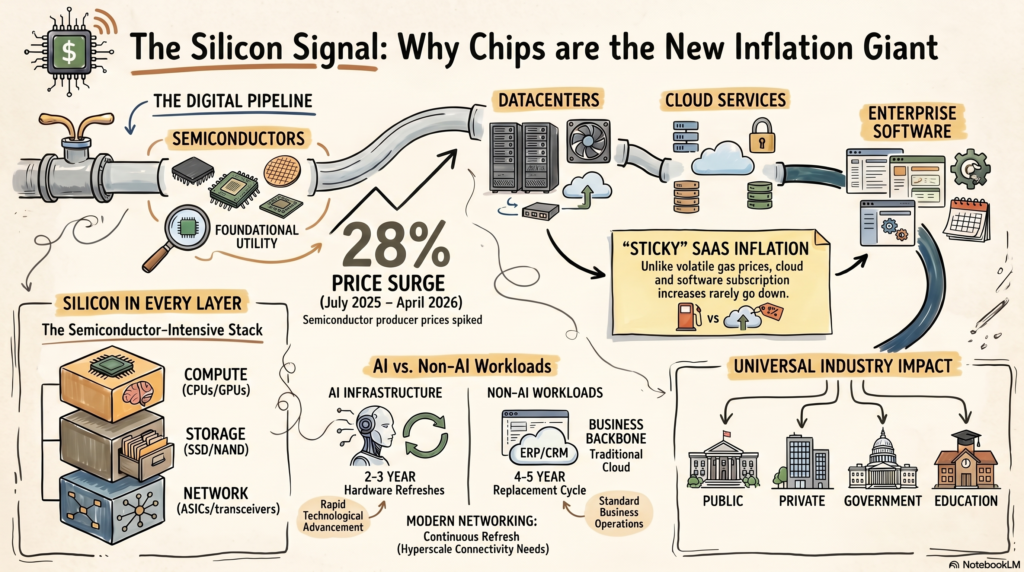
From the July 2025 low to April 2026, semiconductor and electronic component producer prices surged nearly 28%.
That is not the kind of inflation shock typically tied to oil tankers drifting through the Strait of Hormuz or temporary commodity volatility. It is a structural repricing event — one most observers would immediately attribute to the AI gold rush. And they are probably partially correct.
But the implications may reach far beyond AI accelerators themselves.
Semiconductors are no longer just components inside consumer electronics. They are rapidly becoming the foundational infrastructure layer beneath cloud computing, enterprise software, logistics systems, financial platforms, industrial automation, and increasingly the broader economy itself.
If the economics of compute are changing, then the inflation story may be changing with them.
Economists May Be Looking in the Wrong Place
Traditional inflation models were built around industrial-era economics. The classic inflation pipeline looked like this:
Energy -> Transportation -> Manufacturing -> Consumers
That framework makes sense for a physical economy dominated by: fuel, shipping, factories, and commodity production. But the modern economy runs on something else. Increasingly, the real pipeline looks like this:
Semiconductors & Electronics -> Datacenters -> Cloud Services -> Enterprise Software -> Every Industry
This is the inflation architecture of a digital economy. And it changes everything.
Compute Has Become a Foundational Industrial Input
For decades, technology was deflationary. Compute, storage, and bandwidth consistently got cheaper. Infrastructure as a Service (IaaS) and Software as a Service (SaaS) promoted lower total cost of ownership and operational efficiency as core selling points. In many cases that promise proved true. In others, it simply shifted costs from internal IT departments into recurring vendor contracts.
What the broader cloud industry unquestionably established, however, was the normalization of annual price increases embedded inside multi-year customer commitments.
For years, none of this appeared dangerous because the underlying economics of technology remained deflationary. The market internalized the idea that technological progress naturally lowers costs over time.
But what if that assumption is beginning to break?
Part of the answer may lie in how the architecture of cloud infrastructure itself has changed.
Historically, the industry treated compute, storage, and bandwidth as distinct infrastructure categories:
compute meant CPUs and servers,
storage meant hard drives and storage arrays,
bandwidth meant fiber and networking equipment.
Today, all three increasingly collapse into one semiconductor and electronic component intensive stack.
Compute is obviously driven by CPUs, GPUs, accelerators, and memory. But storage is now dominated by NAND flash and SSD controllers. Even bandwidth is no longer “just fiber.” Modern hyperscale networking depends on switching ASICs, optical transceivers, packet processors, NICs, DSPs, and routing silicon. The intelligence layer of the modern internet is semiconductor-driven.
The result is that cloud infrastructure has quietly become an enormous assembly of semiconductor and electronic component based systems connected by glass.
And cloud infrastructure is no longer a niche industry. It is becoming the operational backbone of the global economy.
Payroll systems, logistics platforms, ERP software, CRM systems, healthcare infrastructure, and financial platforms now run inside hyperscale datacenters. These are not speculative AI workloads. They are ordinary, everyday business operations that increasingly depend on semiconductor-intensive infrastructure.
This matters because hyperscalers are entering a perpetual hardware replacement cycle.
That is why a sustained rise in semiconductor and electronic component producer prices matters. If these input costs remain elevated — or continue rising — the effects will eventually work their way through the cloud stack itself, placing upward pressure on SaaS, IaaS, AI inference, and enterprise software pricing.
Not immediately. Hyperscalers hedge aggressively, negotiate long-term supply contracts, and amortize infrastructure investments over years. But producer-price inflation at the hardware layer rarely disappears permanently. Eventually, it surfaces somewhere in the economics of the digital economy.
The Economics Nobody Wants to Talk About
When people discuss AI infrastructure, they focus on model capabilities.
But the economic story is much larger. Google Cloud recently reported:
$20 billion in quarterly revenue,
63% year-over-year growth,
A staggering $462 billion contract backlog
That backlog may be the most important number.
Why?
Because it signals that corporations are committing themselves to long-duration cloud dependence.
These are not experimental workloads or simple eliminations of “server closets” anymore. Cloud infrastructure is becoming mandatory infrastructure. And mandatory infrastructure eventually gains pricing power.
The Replacement Cycle Problem
The semiconductor story becomes even more interesting once you examine hardware replacement cycles. Traditional enterprise servers were typically replaced every 4–5 years. That cycle roughly holds true for the racks of compute infrastructure that powers IaaS and SaaS offerings. AI infrastructure may need replacement every 2–3 years — possibly even faster. The result has been and will continue to be growing and persistent semiconductor demand. Not cyclical demand. Not temporary demand. Permanent demand.
What Happens If Compute Stops Being Deflationary?
This is the macroeconomic question sitting quietly beneath the surface of the semiconductor data. What happens if compute itself becomes inflationary?
The Bureau of Labor Statistics has been tracking Semiconductor as a separate price index since 1984. For those who lived it, you remember the story as prices came down and the economy digitized. The financial crisis of 2008 did not have material impact nor did the post COVID recovery era.
Enter late 2025 and the start of 2026 and semiconductor returns to mid-2000 levels as if it went through an overnight time machine! The difference is that the number of business critical corporate and government workloads that have been migrated to the cloud in the last 20 years has been exponential.
To net it out, rising semi-conductor costs lead to rising cloud infrastructure cost. These costs are the inputs that will drive up SaaS software operating costs and find their way financials just about every sector of the economy both private and public.
The result is a new kind of inflation transmission mechanism. This will not taking place through gasoline pumps but through recurring software invoices. And unlike commodity spikes, SaaS inflation is sticky. Once enterprise subscription pricing rises, it rarely falls.
The New Inflation Utility
Electricity became a universal industrial utility in the 20th century. Compute may be becoming the equivalent utility of the 21st century. If so, semiconductors are no longer just components. They are upstream economic infrastructure. Which means semiconductor pricing may increasingly behave less like a cyclical technology sector and more like a foundational inflation input.
That possibility is hiding in plain sight inside the producer-price data. Yet, the news headlines are still talking about the price of diesel. The next inflation giant may already be sitting quietly inside the datacenter.
As software matures, progress increasingly comes from refinement rather than expansion.
New features remain important, but long-term usability often depends on something less visible: consistency. Users should be able to trust that commands behave predictably, that metadata is presented correctly, and that edge cases are handled without surprises.
Version 1.1.5 focuses on exactly those areas.
This release improves alias management, strengthens citation presentation, resolves structured output edge cases, and closes several correctness gaps discovered during real-world usage.
Together, these changes make RESERVE a more reliable platform for everyday economic data workflows.
Aliases Gain Context
Aliases have always provided a convenient way to create memorable shortcuts for frequently used series.
With v1.1.5, aliases become more than simple mappings.
Users can now attach optional notes when creating aliases:
reserve alias set CPI CPIAUCSL --note "Headline CPI inflation"
Alias metadata now supports:
Required series identifiers
Optional user-authored notes
Richer listing and display behavior
The result is a lightweight documentation layer that allows users to capture intent directly alongside their shortcuts.
As collections of aliases grow, that additional context becomes increasingly valuable.
A name can tell you what something is.
A note can remind you why it matters.
Citations Should Be Predictable
Previous releases introduced citation-aware data handling as part of RESERVE’s broader commitment to responsible economic data stewardship.
Version 1.1.5 continues that effort by improving how citations are presented across observation commands.
Table output now uses a consistent citation model:
Single-source results produce a single Source footer
Multi-source results produce a consolidated Sources footer
Duplicate source entries are automatically removed
Most users will simply notice cleaner output.
More importantly, citation behavior is now predictable regardless of whether a workflow involves one series or many.
Consistency reduces ambiguity and helps ensure attribution remains visible as analysis becomes more complex.
Structured Output Should Stay Structured
One of the most important fixes in this release addresses a subtle but significant interoperability issue.
Certain economic series contain missing observations represented internally as NaN values.
When exported as JSON, these values could previously trigger errors such as:
json: unsupported value: NaN
Version 1.1.5 now converts missing observation values to JSON null.
This change aligns RESERVE output with standard JSON expectations and improves compatibility with downstream tools, scripts, databases, and AI workflows.
The principle is straightforward:
Structured output should remain valid structured output, even when the underlying data contains gaps.
Stronger Alias Ownership Semantics
Several fixes in this release improve how aliases behave across local and user-level configuration files.
Alias deletion now correctly removes entries from the configuration file that actually owns the alias, avoiding situations where merged configuration views could make ownership unclear.
Collision detection has also been strengthened.
When upstream validation services experience transient failures, alias creation now fails closed rather than assuming success.
These changes prioritize correctness over convenience and help prevent subtle configuration inconsistencies from accumulating over time.
Preserving Compatibility
As configuration models evolve, existing users should not be forced into disruptive migrations.
To support that goal, RESERVE now tolerates legacy string-based alias definitions during reads while continuing to write the newer structured format.
This allows older configurations to remain functional while gradually moving users toward the canonical representation.
The migration path becomes effectively automatic.
Small Improvements, Bigger Reliability
Many releases are remembered for a single headline feature.
Version 1.1.5 is different.
Its value comes from dozens of small improvements that collectively strengthen the user experience.
Aliases now carry richer context.
Citation behavior is more consistent.
Structured outputs are more reliable.
Configuration ownership is clearer.
Compatibility is stronger.
None of these changes dramatically alter what RESERVE can do.
They improve confidence in how RESERVE does it.
And for a tool intended to support serious economic analysis, that confidence matters.
Ground beef comes in a wide range of varieties, with pricing influenced by factors such as fat content, grading quality, and premium options like grass-fed beef. Every one of these characteristics affects the final retail price consumers see at the grocery store.
Historically, ground beef prices have moved in cycles, rising and falling alongside broader commodity markets, cattle supply, feed costs, transportation expenses, and consumer demand. But in recent years, something has clearly changed. The long-term trend no longer looks cyclical—it looks relentless. Prices keep climbing, and consumers are feeling it every time they walk through the meat aisle.
What was once considered one of the most affordable and dependable protein options for American families is rapidly becoming another example of persistent food inflation. And according to the data, this isn’t just perception—it’s measurable reality.
Ground Beef Price Data
Two Federal Reserve Economic Data (FRED) series publish monthly average retail pricing data for ground beef:
“Average Price: Ground Beef, Lean and Extra Lean” (APU0000703113)
These datasets provide a long-term view into how dramatically retail beef prices have changed over time. One of the easiest ways to locate the series is by using the FRED search function or RESERVE search command:
This search reveals these two series along with other related commodity oriented data series.
Examining the Trend
Price increases are best understood visually. While these series can certainly be exported into a spreadsheet for graphing and further analysis, RESERVE already provides both a powerful transform command set and built-in ASCII charting capabilities.
The transform commands are especially useful for converting raw data into a more macro-level view of the underlying trend. Since both ground beef datasets are published monthly, aggregating the data into quarterly or yearly intervals provides a much clearer picture of the long-term direction of prices while reducing short-term noise.
One of RESERVE’s strengths is composability. The results from the original search can be passed directly into the transform command set and then piped into the charting commands for visualization. The result is shown below:
The grade-school explanation for rising prices usually simplifies inflation down to basic supply and demand. In reality, modern economies are tightly interconnected ecosystems where countless variables interact simultaneously—each with its own supply constraints, demand pressures, and downstream effects.
Ground beef prices are a perfect example. Retail pricing is influenced not only by consumer demand, but also by cattle inventory levels, feed costs, fuel prices, transportation expenses, labor markets, interest rates, weather conditions, and even import/export dynamics. Every layer of the supply chain contributes pressure to the final price consumers see at the grocery store.
One of the strengths of the FRED system is that this data is publicly accessible for both hobbyists and researchers to explore. For anyone interested in understanding the forces driving the long-term rise in ground beef prices, RESERVE search makes it possible to discover and analyze datasets covering everything from hay and diesel costs to cattle inventories, beef production, and international trade flows.
Marketplace, the popular economics podcast, has built a reputation for making complex economic topics accessible to everyday listeners. Much of that appeal comes from host Kai Ryssdal, whose mix of sharp insight, humor, and storytelling makes even the driest data surprisingly entertaining.
On May 7, 2026, the Marketplace episode contained a segment titled “Measuring Economic Demand.” The episode focused on a lesser-known economic indicator — Final Sales to Private Domestic Purchasers. The point was to explain why economists often view it as a cleaner measure of underlying demand than headline GDP.
This post picks up where Marketplace left off. Using RESERVE, readers can explore the data themselves, track the series over time, and dig deeper into the economic story behind the numbers.
The segment also sparked an idea for a new RESERVE feature — one I’ll introduce at the end of this post.
What Did Kai Actually Say
In the Marketplace segment, Kai Ryssdal walked listeners through the basic building blocks of Gross Domestic Product (GDP): consumer spending, business investment, government spending, and net exports.
Then, in classic Kai fashion, he slowed things down and carefully unpacked a lesser-known measure: Final Sales to Private Domestic Purchasers.
At its core, the metric strips away some of GDP’s noisier components — namely net exports, government spending, and inventory swings. The intent is to focus more directly on underlying private-sector demand in the U.S. economy.
Rather than using the finalized quarterly GDP reports, the segment focused on the advance estimates, the first look economists get at quarterly economic growth data.
To find this series in RESERVE, use the following search command:
reservesearch"Final Sales to Private"Searchresultsfor:"Final Sales to Private"+--------------------+----------------------------------------------------+------+----------------------+------------------------+|ID|TITLE|FREQ|UNITS|LASTUPDATED|+--------------------+----------------------------------------------------+------+----------------------+------------------------+|LB0000031Q020SBEA|RealFinalSalestoPrivateDomesticPurchasers|Q|Bil.of2017US $ |2026-04-3007:48:54-05||PB0000031Q225SBEA|Realfinalsalestoprivatedomesticpurchasers|Q|%Chg.fromPrece...|2026-04-3007:48:33-05||PE0000031Q156NBEA|RealFinalsalestoprivatedomesticpurchasers|Q|%Chg.fromQtr....|2026-04-3007:48:30-05||PB0000031A225NBEA|Realfinalsalestoprivatedomesticpurchasers|A|%Chg.fromPrece...|2026-03-1307:49:16-05||LA0000031Q027SBEA|FinalSalestoPrivateDomesticPurchasers|Q|Bil.of $ |2026-04-3007:49:20-05||LA0000031A027NBEA|Finalsalestoprivatedomesticpurchasers|A|Bil.of $ |2026-04-0907:53:06-05||FINSALESDOMPRIVPUR|NowcastforRealFinalSalesofPrivateDomesti...|Q|%Chg.atAnnual...|2026-05-0811:02:58-05||GOR|GrossOutputbyIndustry:RetailTrade|Q|Bil.of $ |2026-04-0907:34:48-05||A811RC2Q027SBEA|Ratiosofprivateinventoriestofinalsalesof...|Q|%|2026-04-3007:50:53-05||PA0000031Q225SBEA|Finalsalestoprivatedomesticpurchasers,cur...|Q|%Chg.fromPrece...|2026-04-3007:48:25-05||PA0000031A225NBEA|Finalsalestoprivatedomesticpurchasers,cur...|A|%Chg.fromPrece...|2026-02-2007:46:57-06|
The series ID for the quarterly updated version of Real Final Sales to Private Domestic Purchasers is PB0000031Q225SBEA . Note, that if this series is examined with the META SERIES command and formatted in JSON, RESERVE will give the user almost verbatim Kai’s explanation (minus the humor). See the NOTES field for the definition.
reservemetaseriesPB0000031Q225SBEA--formatjson{"kind":"series_meta","generated_at":"2026-05-09T15:54:44.926228-05:00","command":"meta series PB0000031Q225SBEA","data": [{"id":"PB0000031Q225SBEA","title":"Real final sales to private domestic purchasers","observation_start":"1947-04-01","observation_end":"2026-01-01","frequency":"Quarterly","frequency_short":"Q","units":"Percent Change from Preceding Period","units_short":"% Chg. from Preceding Period","seasonal_adjustment":"Seasonally Adjusted Annual Rate","seasonal_adjustment_short":"SAAR","last_updated":"2026-04-30 07:48:33-05","popularity":38,"notes":"BEA Account Code: PB000003\n\nFinal sales to domestic purchasers less government consumption expenditures and gross investment. \nA Guide to the National Income and Product Accounts of the United States (NIPA) - (http://www.bea.gov/national/pdf/nipaguid.pdf)","source_name":"Bureau of Economic Analysis","copyright_status":"public_domain_citation_requested","citation_text":"Source: Bureau of Economic Analysis via FRED","usage_allowed_commercial":true,"usage_allowed_educational":true,"usage_allowed_personal":true,"raw_rights_tags": ["public domain: citation requested" ],"last_rights_check_at":"2026-05-09T20:53:26.738003Z","fetched_at":"2026-05-09T20:53:26.738011Z"} ],"stats":{"cache_hit":false,"duration_ms":0,"items":1}}
Also note in the original search that pulling data from the affiliated series PB0000031Q225SBEA will provide the percentage change since last published series which is that 2.5% number Kai referenced.
The point of this exercise is that podcast like Marketplace offer incredible insight and perspective on economics data. If a listener finds this interesting, they can use RESERVE and their free API key from FRED® to explore the topic even further. That is the point of RESERVE–lowering the barrier of entry to the over 800 data series made accessible by the Federal Reserve Bank of St. Louis.
What Upcoming Feature Did Kai Inspire?
In Kai fashion, he spoke the words “Final Sales to Private Domestic Purchasers” very slowly. Why? It’s a mouthful that’s why. However, the corresponding series data he referenced is not only a mouth full but it is cryptic! “PB0000031Q225SBEA”
Coming in RESERVE 1.1.5 the intent is to introduce an ALIAS command that would support the following:
reservealiassetFSPDPPB0000031Q225SBEA--note"Real Final Sales Dom. Producers "reservealiaslistreservealiasgetFSPDPreservealiasdeleteFSPDP